
With the advancement of deep learning such as convolutional neural network (i.e., ConvNet) [1], computer vision becomes a hot scientific research topic again. One of the main goals of computer vision nowadays is to use machine learning (especially deep learning) to train computers to gain a human-level understanding of digital images, texts, or videos.
With its widespread use, ConvNet becomes the de facto model for image recognition. As described in [1], generally speaking, there are two approaches for using ConvNet for computer vision:
As shown in the following diagram, a ConvNet model consists of two parts: a convolutional base and a fully connected classifier.
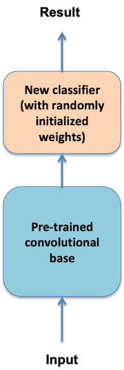
Figure 1: Typical scenario of ConvNet transfer learning.
The ConvNet transfer learning can be further subdivided into three methods:
Method 2 is used in this article for multi-input model transfer learning.
The main idea behind transfer learning can be used to supervise ConvNet and other deep learning algorithms such as the unsupervised word embedding models for natural language processing (NLP)[4].
There are two popular pre-trained word embedding models: word2vec and GloVe [3]. Like the word2vec-keras model used in [4], these pre-trained word embedding models are usually combined with other supervised deep learning algorithms such as the recurrent neural network (RNN) LSTM for NLP such as text classification [4].
A ConvNet model or an NLP model (e.g., a combination of word embedding with LSTM) can be used separately to solve many interesting problems in computer vision and NLP. As to be shown in this article, these different types of models can also be combined in various ways [1] to form more powerful models to address more challenging problems such as insurance claim process automation that require not only the capability of image recognition but also natural language (e.g., texts) understanding.
This article uses an interesting but challenging dataset in Kaggle, Challenges in Representation Learning: Multi-modal Learning [2], to present a new multi-input transfer learning model that combines two input models with a fully connected classification layer for both image recognition and word tag recognition at the same time (see Figure 2).
The main idea behind the new multi-input model is to translate image and word tag recognition into a machine learning classification problem, that is, determining whether or not a given image matches a given set of word tags (0-No, 1-Yes).
After the Kaggle dataset of image files and word tag files [2] has been downloaded onto a local machine, the code below can be used to build and shuffle the lists of image file names and related word tag file names. There are 100,000 image files and 100,000 corresponding word tag files in the dataset for training purposes.
original_dataset_dir = './multi_task_learning/data/ESPGame100k'
base_dataset_dir = './multi_task_learning/data/ESPGame100k_small'

original_label_path = original_dataset_dir + '/labels'
original_label_files = [f for f in listdir(original_label_path) if isfile(join(original_label_path, f))]

original_image_path = original_dataset_dir + '/thumbnails'
original_image_files = [f for f in listdir(original_image_path) if isfile(join(original_image_path, f))]

original_image_files = np.array(original_image_files)
original_label_files = np.array(original_label_files)

dataset_size = original_label_files.shape[0]
perm = np.arange(dataset_size)
 np.random.shuffle(perm)
 original_image_files = original_image_files[perm]
 original_label_files = original_label_files[perm]
To train the new multi-input model on a laptop within a reasonable amount of time (a few hours), I randomly selected 2,000 images and corresponding 2,000-word tag files for model training for this article:
if not os.path.isdir(base_dataset_dir):
     os.mkdir(base_dataset_dir)

 small_label_path = os.path.join(base_dataset_dir, 'labels')
 small_image_path = os.path.join(base_dataset_dir, 'thumbnails')
 if not os.path.isdir(small_label_path):
     os.mkdir(small_label_path)
 if not os.path.isdir(small_image_path):
     os.mkdir(small_image_path)

for fname in original_label_files[:2000]:
     src = os.path.join(original_label_path, fname)
     dst = os.path.join(small_label_path, fname)
     shutil.copyfile(src, dst)

for fname in original_label_files[:2000]:
     img_fname = fname[:-5]
     src = os.path.join(original_image_path, img_fname)
     dst = os.path.join(small_image_path, img_fname)
     shutil.copyfile(src, dst)
The code below is to load the 2,000 image tag file names and the corresponding 2,000-word tags into Pandas DataFrame:
label_map = {'label_file' : [], 'word_tags' : []}
 for fname in listdir(small_label_path):
     f = join(small_label_path, fname)
     if isfile(f):
         f = open(f)

label_map['label_file'].append(fname)
         line = f.read().splitlines()
         label_map['word_tags'].append(line)
 label_df = pd.DataFrame(label_map)
 label_df.head()

Similarly to [4], a textual data preprocessing procedure is included in the Jupyter notebook [5] to perform minimum data preprocessing such as removing stop words and numeric numbers in case it makes a significant difference:

As described in [4], the impact of textual data preprocessing is insignificant, and thus the raw word tags without preprocessing are used for model training in this article.
The diagram below shows that the new multi-input transfer learning model uses the pre-trained ConvNet model VGG16 for receiving and handling images and a new NLP model (a combination of the pre-trained word embedding model GloVe and Keras LSTM) for receiving and handling word tags. These two input models are merged first and then combined with a fully connected output classification model that uses both the image recognition model output and the NLP model output to determine whether or not an input pair of an image and a set of word tags is a match (0-No, 1-Yes).
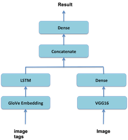
Figure 2: The architecture of the new deep learning model for multi-input models transfer learning.
As shown in Figure 2, the new multi-input transfer learning model uses the pre-trained ConvNet model VGG16 for image recognition. The VGG16 model has already been included in the Keras library. The following code from [1] is used to combine the VGG16 convolutional base with a new fully-connected classifier to form a new image recognition input model:
from keras.applications import VGG16

image_input = Input(shape=(150, 150, 3), name='image')
vgg16 = VGG16(weights='imagenet',
                   include_top=False,
                   input_shape=(150, 150, 3))(image_input)
x = layers.Flatten()(vgg16)
x = layers.Dense(256, activation='relu')(x)
As shown in Figure 2, the new multi-input transfer learning model uses the pre-trained word embedding model GloVe [3] for converting word tags into compact vectors. Once the GloVe dataset [3] has been downloaded to the local machine, the following code from [1] can be used to load the word embedding model into memory:
glove_dir = './multi_task_learning/data/'

embeddings_index = {}
f = open(os.path.join(glove_dir, 'glove.6B.100d.txt'))
for line in f:
     values = line.split()
     word = values[0]
     coefs = np.asarray(values[1:], dtype='float32')
     embeddings_index[word] = coefs
f.close()
As it can be seen in Figure 2, the GloVe word embedding is combined with Keras LSTM to form a new NLP input model for predicting/recognizing word tags:
tag_input = Input(shape=(None,), dtype='int32', name='tag')
embedded_tag = layers.Embedding(max_words, embedding_dim)(tag_input)
encoded_tag = layers.LSTM(512)(embedded_tag)
Once the new image recognition input model and the new NLP input model have been created, the following code can combine them with a new output classifier into one multi-input transfer learning model:
concatenated = layers.concatenate([x, encoded_tag], axis=-1)
output = layers.Dense(1, activation='sigmoid')(concatenated)model = Model([image_input, tag_input], output)
model.summary()
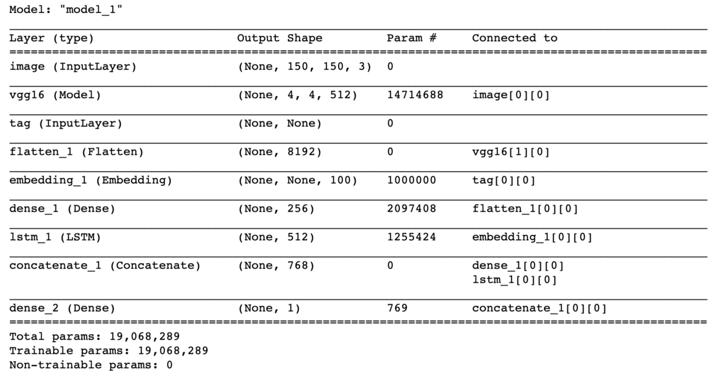
As described in [1], both the pre-trained VGG16 convolutional base and the GloVe word embedding layer must be frozen so that the pre-trained weights of those models will not be modified during the new multi-input model training:
# model.layers[1].trainable = False # freeze VGG16
model.layers[4].set_weights([embedding_matrix])
model.layers[4].trainable = False # freeze GloVe word embedding
However, regarding the VGG16 convolutional base, it is interesting to note that I tried both ways (frozen and not frozen) but did not see a significant difference in terms of model training time or model prediction results.
The original Kaggle training dataset includes only the correct pairs of images and corresponding word tags. Each correct pair is labeled as 1 (match) in this article (also see the code below). To create a balanced dataset, the following code creates 2,000 incorrect pairs of images and word tags in addition to the existing 2,000 correct pairs of images and word tags. For simplicity, this is achieved by pairing each (say Image i) of the selected 2,000 images with the word tags of the following image file (i.e., word tags of Image i+1).
import cv2

dim = (150, 150)
 X_image_train = []
 X_tag_train = tag_data
 y_train = []

for fname in listdir(small_image_path):
     fpath = os.path.join(small_image_path, fname)
     im = cv2.imread(fpath)
     im_resized = cv2.resize(im, dim, interpolation = cv2.INTER_AREA)
     X_image_train.append(im_resized)
     y_train.append(1)

# add incorrect image and tag pairs
num_negative_samples = len(y_train)
for i in range(num_negative_samples):
     image = X_image_train[i]
     X_image_train.append(image)
     j = (i + 1) % num_negative_samples # get a different tag
     tag = X_tag_train[j]
     X_tag_train = np.append(X_tag_train, tag)
     y_train.append(0)
There are 4,000 pairs of images and word tags in total, 2,000 correct pairs, and 2,000 incorrect pairs.
Each of the image word tags needs to be encoded as an integer, and each list/sequence of word tags needs to be converted into a sequence of integer values before the word tags can be consumed by the word embedding model. This is achieved as follows by using and modifying the code in [1]:
from keras.preprocessing.text import Tokenizer
from keras.preprocessing.sequence import pad_sequences

maxlen = 100
training_samples = num_of_samples
tag_vocabulary_size = 10000
max_words = tag_vocabulary_size
num_of_samples = label_df.shape[0]

tokenizer = Tokenizer(num_words=max_words)
texts = []
for tag_list in label_df_clean['word_tags']:
     texts.append(' '.join(tag_list))
tokenizer.fit_on_texts(texts)
sequences = tokenizer.texts_to_sequences(texts)
word_index = tokenizer.word_index
print('Found {} unique tokens'.format(len(word_index)))
tag_data = pad_sequences(sequences, maxlen=maxlen)
The resulting image and word tag training datasets are converted into Numpy arrays and shuffled for model training:
X_image_train = np.array(X_image_train)
X_tag_train = np.array(X_tag_train)
y_train = np.array(y_train)
perm = np.arange(y_train.shape[0])
np.random.shuffle(perm)
X_image_train = X_image_train[perm]
X_tag_train = X_tag_train[perm]
y_train = y_train[perm]
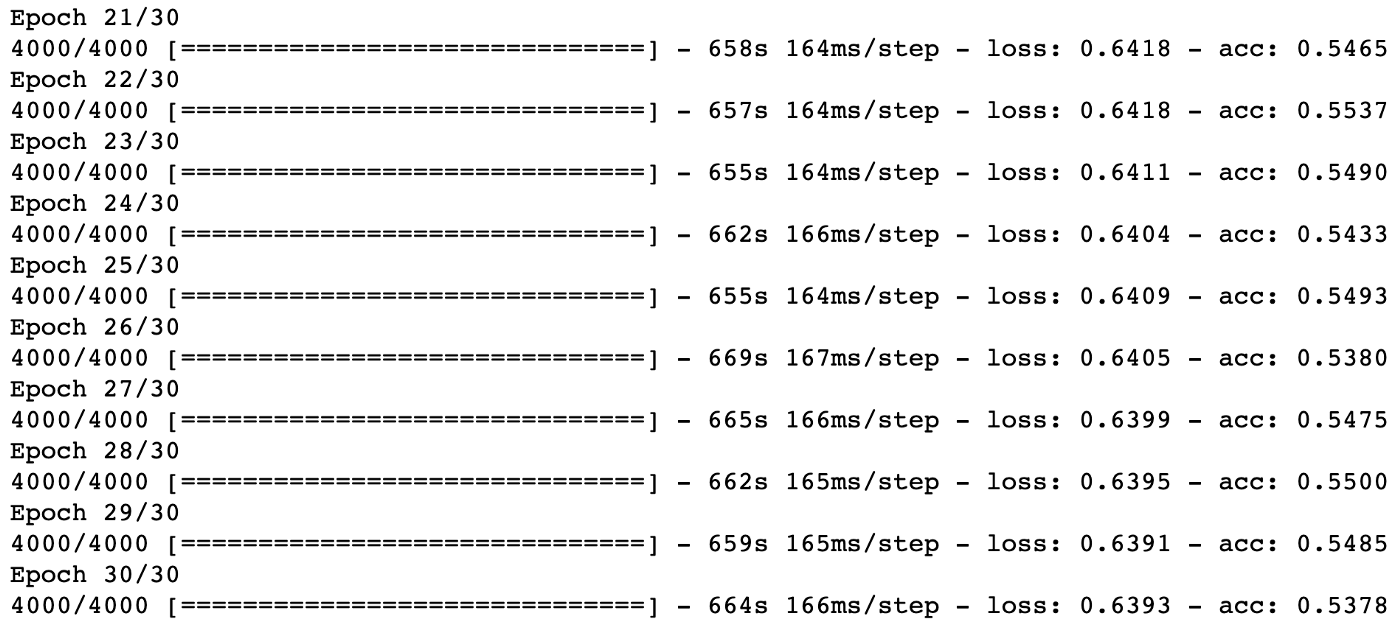
The new multi-input model is compiled and trained as follows with only 30 epochs and 4,000 balanced pairs of images and word tags:
model.compile(optimizer='rmsprop', loss='binary_crossentropy', metrics=['acc'])
model.fit([X_image_train, X_tag_train], y_train, epochs=30, batch_size=64)
As shown below, the private testing dataset in [2] includes 500 images, and each image is associated with two sets of word tags:

Given an image in the testing dataset, the new multi-input transfer learning model needs to predict which of the given two sets of word tags matches the image.
The following code is to load the testing images into memory:
dim = (150, 150)
X_image_test = []

for fname in listdir(test_image_dir):
     fpath = os.path.join(test_image_dir, fname)
     im = cv2.imread(fpath)
     im_resized = cv2.resize(im, dim, interpolation = cv2.INTER_AREA)
     X_image_test.append(im_resized)
The testing word tags are converted into a sequence of encoded integer values as follows:
tokenizer_test = Tokenizer(num_words=max_words)
texts_1 = []
texts_2 = []
texts_all = []
for tag_list in test_image_label_df['word_tags_1']:
     texts_1.append(' '.join(tag_list))
for tag_list in test_image_label_df['word_tags_2']:
     texts_2.append(' '.join(tag_list))
texts_all.extend(texts_1)
texts_all.extend(texts_2)
tokenizer_test.fit_on_texts(texts_all)
sequences_1 = tokenizer_test.texts_to_sequences(texts_1)
sequences_2 = tokenizer_test.texts_to_sequences(texts_2)

word_index_test = tokenizer_test.word_index
print('Found {} unique tokens in test'.format(len(word_index_test)))
tag_data_test_1 = pad_sequences(sequences_1, maxlen=maxlen)
tag_data_test_2 = pad_sequences(sequences_2, maxlen=maxlen)
The resulting Python arrays of images and word tags are then converted into Numpy arrays and fit into the trained model for prediction:
X_image_test = np.array(X_image_test)
X_tag_test_1 = np.array(tag_data_test_1)
X_tag_test_2 = np.array(tag_data_test_2)
y_predict_1 = loaded_model.predict([X_image_test, X_tag_test_1])
y_predict_2 = loaded_model.predict([X_image_test, X_tag_test_2])
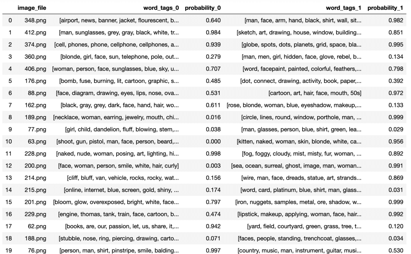
The following table shows the first 20 prediction results:
The following image is Image 201.png in the testing dataset:
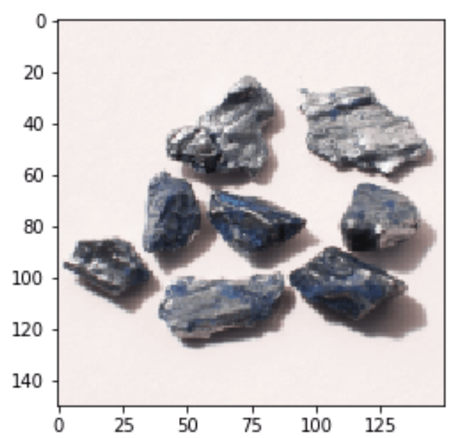
The two associated sets of word tags are as follows:
word-tag-set-0: ['bloom', 'glow', 'overexposed', 'bright', 'white', 'face', 'woman', 'blonde']
word-tag-set-1: ['iron', 'nuggets', 'samples', 'metal', 'ore', 'shadow', 'white', 'grey', 'gray', 'rust', 'shiny']
The model predicts:
word-tag-set-0: probability of 0.797
word-tag-set-1: probability of 0.999
The answer with the higher probability of 0.999 is:
[‘iron’, ‘nuggets’, ‘samples’, ‘metal’, ‘ore’, ‘shadow’, ‘white’, ‘grey’, ‘gray’, ‘rust’, ‘shiny’]
As another positive example, the following is Image 76.png in the testing dataset:
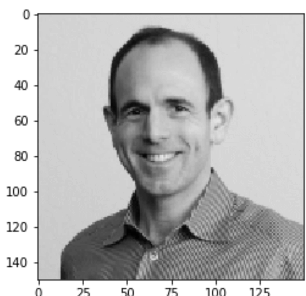
The following are the associated two sets of word tags:
word-tag-set-0: ['person', 'man', 'shirt', 'pinstripe', 'smile', 'balding', 'grey', 'gray']
word-tag-set-1: ['country', 'music', 'man', 'instrument', 'guitar', 'musician', 'person', 'playing', 'watch', 'striped', 'shirt', 'red', 'glasses']
The model predicts:
word-tag-set-0: probability of 0.997
word-tag-set-1: probability of 0.530
The answer with the higher probability of 0.997 is:
[‘person’, ‘man’, ‘shirt’, ‘pinstripe’, ‘smile’, ‘balding’, ‘grey’, ‘gray’]
As a false positive example, the following is Image 189.png in the testing dataset:
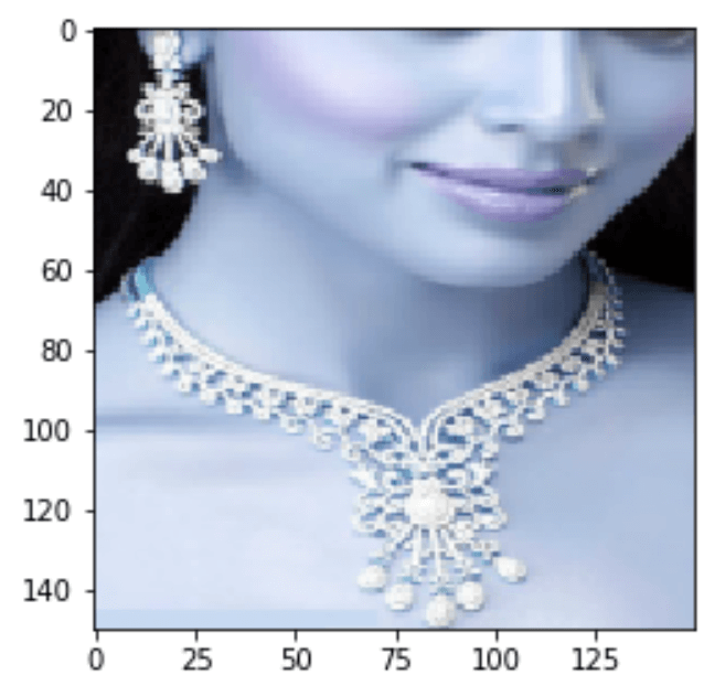
The following are the associated two sets of word tags:
word-tag-set-0: ['necklace', 'woman', 'earring', 'jewelry', 'mouth', 'chin', 'closeup']
word-tag-set-1: ['circle', 'lines', 'round', 'window', 'porthole', 'man', 'face', 'beard', 'person', 'dark', 'shadow']
The model predicts:
word-tag-set-0: probability of 0.016
word-tag-set-1: probability of 0.999
The false-positive answer with the higher probability of 0.999 is:
[‘circle’, ‘lines’, ‘round’, ‘window’, ‘porthole’, ‘man’, ‘face’, ‘beard’, ‘person’, ‘dark’, ‘shadow’]
The testing results above show that even though the new multi-input transfer learning model is trained with only 4,000 pairs of images and word tags and 30 epochs, the model obtained quite reasonable results in terms of accuracy.
However, the model also generated quite some false positives due to model overfitting.
This article presented a new multi-input deep transfer learning model that combines two pre-trained input models (VGG16 and GloVe & LSTM) with a new fully-connected classification layer for recognizing images and word tags simultaneously.
The key point of the new multi-input deep learning method is to translate the problem of image and word tag recognition into a classification problem, that is, determining whether or not a given image matches a given set of word tags (0-No, 1-Yes).
The challenging public dataset in Kaggle, Challenges in Representation Learning: Multi-modal Learning [2], was used to train and evaluate the new model.
The model prediction results demonstrated that the new model performed reasonably well with limited model training (only 30 epochs and 4,000 pairs of images and word tags) for demonstration purposes. However, with no surprise, the model also generated quite some false positives due to model overfitting. This issue can be addressed by training the model with more epochs and more pairs of images and word tags.
A randomly chosen 2,000 training images were not good enough representative of a total of 100,000 available training images. Therefore, the model performance should be improved significantly by increasing training images from 2,000 to a larger size like 10,000.
A Jupyter notebook with all of the source code is available on GitHub [5].
[1] F. Chollet, Deep Learning with Python, Manning Publications Co., 2018
[2] Challenges in Representation Learning: Multi-modal Learning
[3] J. Pennington, R. Socher, C.D. Manning, GloVe: Global Vectors for Word Representation
[4] Y. Zhang, Deep Learning for Natural Language Processing Using word2vec-keras
[5] Y. Zhang, Jupyter notebook in Github